Exercise 4.6
An AR(2) TFP Process And Excess Consumption Volatility
Problem
In this exercise you are asked to show that the SOE-RBC model can predict consumption to be more volatile than output when the productivity shock follows an AR(2) process displaying a hump-shaped impulse response. The theoretical model to be used is the EDEIR model presented in section 4.1.1. Replace the AR(1) process with the following AR(2) specification:
\[ \ln A_{t+1} = 1.42 \ln A_t - 0.43 \ln A_{t-1} + \epsilon_{t+1}, \]
where \(\epsilon_t\) is an i.i.d. random variable with mean zero and standard deviation \(\sigma_\epsilon > 0\). Scale \(\sigma_\epsilon\) to ensure that the predicted standard deviation of output is 3.08, the value predicted by the AR(1) version of this model. Otherwise use the same calibration and functional forms as presented in the chapter.
Download the Matlab files for the EDEIR model from http://www.columbia.edu/~mu2166/closing.htm. Then modify them to accommodate the present specification.
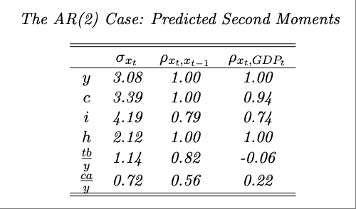
Produce a table displaying the unconditional standard deviation, serial correlation, and correlation with output of output, consumption, investment, hours, the trade-balance-to-output ratio, and the current-account-to-output ratio.
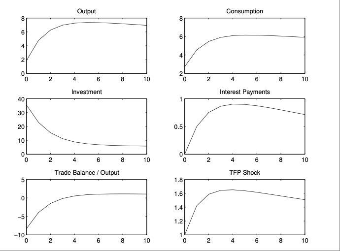
Produce a 3 × 2 figure displaying the impulse responses of output, consumption, investment, hours, the trade-balance-to-output ratio, and TFP to a unit innovation in TFP.
Compare and contrast the predictions of the model under the AR(1) and the AR(2) TFP processes. Provide intuition.
Answer
📥 Download Matlab Code (4_6_code.zip)
1.
2.
3.
Relative to the AR(1) specification (as in Table 4.2 and Figure 4.1), the AR(2) TFP process generates a more persistent shock. This increased persistence is present in the responses of output, consumption, investment and hours to shocks. The trade balance remains countercyclical. Comparing the standard deviations and correlations across models (while holding output volatility constant by construction), the AR(2) model yields more volatile consumption, significantly less volatile investment, and reduced volatility in the trade balance and current account. Serial correlation increases across all variables, as expected under a more persistent shock process. Additionally, output becomes more strongly correlated with consumption, investment, and hours worked, while its correlation with the trade balance and current account declines.