Exercise 4.5
Complete Asset Markets and External Shocks
Problem
Consider the CAM model of section 4.9. Suppose that the productivity factor \(A_t\) is constant and normalized to 1. Replace the equilibrium condition \(U_c(c_t, h_t) = \psi_{CAM}\) with the expression
\[ U_c(c_t, h_t) = x_t, \]
where \(x_t\) is an exogenous and stochastic random variable, which can be interpreted as an external shock. Assume that the external shock follows a process of the form
\[ \hat{x}_t = \rho \hat{x}_{t-1} + \epsilon_t, \quad \epsilon_t \sim N(0, \sigma_\epsilon^2), \]
where \(\hat{x}_t \equiv \ln(x_t / \bar{x})\), and \(\bar{x}\) denotes the nonstochastic steady-state level of \(x_t\). Let \(\rho = 0.9\) and \(\sigma_\epsilon = 0.02\). Calibrate all other parameters of the model following the calibration of the CAM model presented in section 4.9. Finally, set the steady-state value of \(x_t\) in such a way that the steady-state level of consumption equals the level of steady-state consumption in the version of the CAM model studied in the main text.
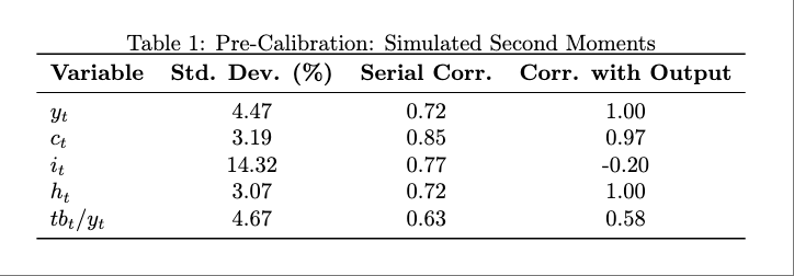
Produce a table displaying the unconditional standard deviation, serial correlation, and correlation with output of \(\hat{y}_t\), \(\hat{c}_t\), \(\hat{i}_t\), \(\hat{h}_t\), and \(tb_t / y_t\).
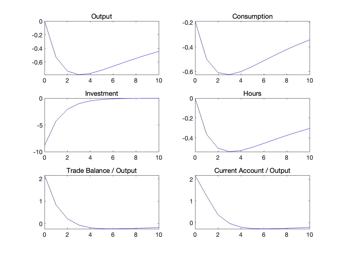
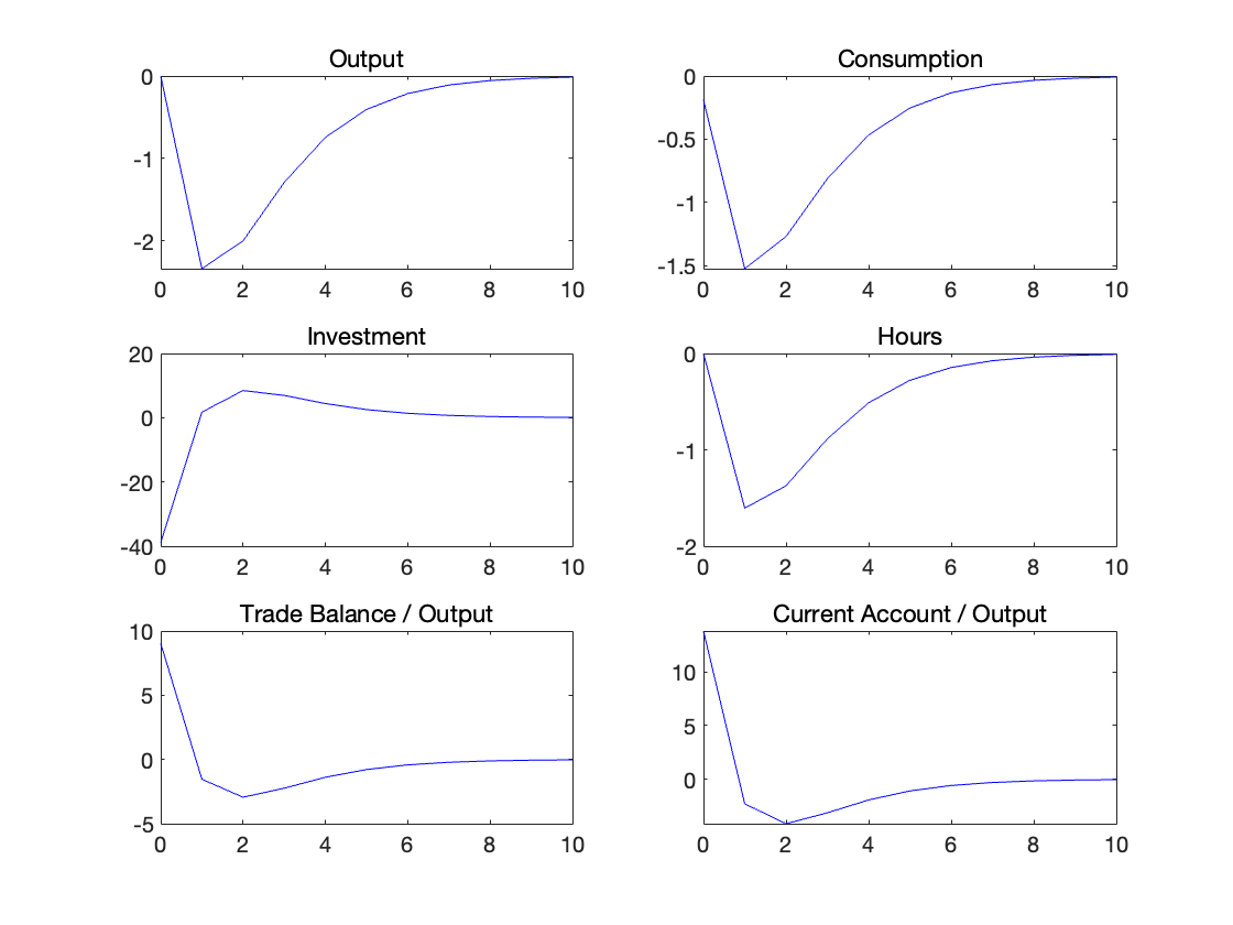
Produce a figure with five plots depicting the impulse responses to an external shock (a unit innovation in \(\epsilon_t\)) of \(\hat{y}_t\), \(\hat{c}_t\), \(\hat{i}_t\), \(\hat{h}_t\), and \(tb_t / y_t\).
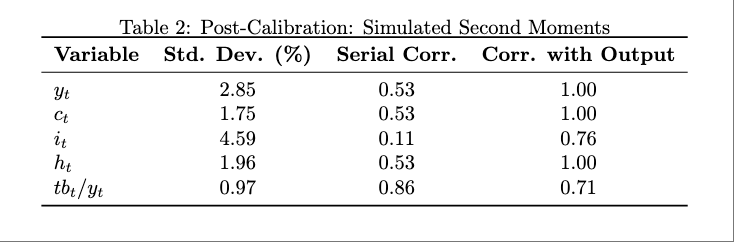
Now replace the values of \(\rho\) and \(\sigma_\epsilon\) given above with values such that the volatility and serial correlation of output implied by the model are the same as those reported for the Canadian economy in table 4.2. Answer questions 1 and 2 using these new parameter values.
Based on your answer to question 3, evaluate the ability of external shocks (as defined here) to explain business cycles in Canada.
Answer
📥 Download Matlab Code (4_5_code.zip)
1.
2.
3.
4.
The model matches some key features of Canadian business cycles reasonably well. The volatility of output is calibrated to match the data (2.85% vs. 2.81%), and the standard deviations of consumption (1.75%) and hours worked (1.96%) are plausible and highly correlated with output.
However, the model fails to generate realistic investment dynamics. The volatility of investment is only 4.59%, which is much lower than in the data, and its serial correlation is just 0.11, indicating almost no persistence. This suggests that the model lacks frictions such as capital adjustment costs.
The trade-balance-to-output ratio shows high persistence (0.86) and moderate volatility (0.97%), which are consistent with data from small open economies.
Overall, the model performs well in capturing output, consumption, and external balance behavior, but does poorly in explaining investment volatility and persistence.