Exercise 4.11
A Model of the U.S.-Canadian Business Cycle
Problem
Consider a world with two economies, Canada and the United States, indexed by \(i=Can,US\), respectively. Suppose that both economies are populated by a large number of identical households with preferences given by
\[ E_0 \sum_{t=0}^{\infty} \beta^t \frac{\left[ c^i_t - \frac{ (h^i_t)^{\omega}}{\omega}\right]^{1-\sigma} - 1}{1 - \sigma}, \]
where \(c^i_t\) and \(h^i_t\) denote, respectively, consumption and hours worked in country \(i\) in period \(t\). In both countries, households operate a technology that produces output, denoted \(y^i_t\), using labor and capital, denoted \(k^i_t\). The production technology is Cobb-Douglas and is given by
\[ y^i_t = A^i_t (k^i_t)^{\alpha} (h^i_t)^{1-\alpha}, \]
where \(A^i_t\) denotes a productivity shock in country \(i\), which evolves according to the following AR(1) process:
\[ \ln A^i_{t+1} = \rho^i \ln A^i_t + \eta^i \epsilon^i_{t+1}, \]
where \(\epsilon^i_t\) is an i.i.d. innovation with mean zero and variance one, and \(\rho^i\) and \(\eta^i\) are country-specific parameters. Both countries produce the same good. The evolution of capital obeys the following law of motion:
\[ k^i_{t+1} = k^i_t + \frac{1}{\phi^i} \left[ \left( \frac{i^i_t}{\delta k^i_t} \right)^{\phi^i} - 1 \right] \delta k^i_t, \]
where \(i^i_t\) denotes investment in country \(i\), and \(\phi^i\) is a country-specific parameter.
Assume that asset markets are complete and that there exists free mobility of goods and financial assets between the United States and Canada, but that labor and installed capital are immobile across countries. Finally, assume that Canada has measure zero relative to the United States, so that the latter can be modeled as a closed economy.
Consider the business cycle regularities for Canada for the period 1960–2011 shown in Exercise 4.10. The following table displays observed standard deviations, serial correlations, and correlations with output for the United States for 1960–2011. The data are annual and are expressed in per capita terms. The series \(y\), \(c\), and \(i\) are in logs, and the series \(tb/y\) is in levels. All series were quadratically detrended. Standard deviations are measured in percentage points.
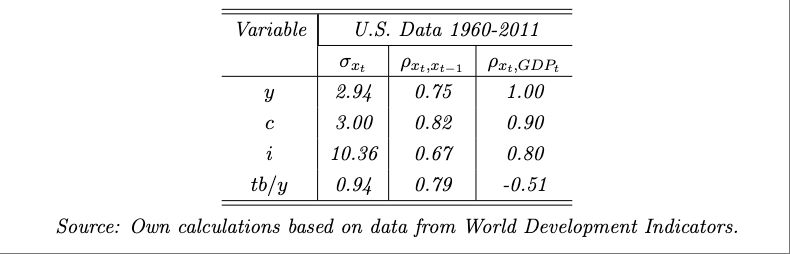
Source: Own calculations based on data from World Development Indicators.
Calibrate the model as follows. Assume that the deterministic steady-state levels of consumption per capita are the same in Canada and the United States. Set \(\beta = 1/1.04\), \(\sigma = 2\), \(\omega = 1.455\), \(\alpha = 0.32\), and \(\delta = 0.10\). Set the remaining six parameters, \(\rho^i\), \(\eta^i\), and \(\phi^i\), for \(i = \text{Can, US}\), to match the observed standard deviations and serial correlations of output and the standard deviations of investment in Canada and the United States. Use a distance minimization procedure as in exercise 4.8.
Approximate the equilibrium dynamics up to first order. Produce the theoretical counterparts of the two tables showing Canadian and U.S. business-cycle regularities.
Comment on the ability of the model to explain observed business cycles in Canada and the United States.
Plot the response of Canadian output, consumption, investment, hours, and the trade-balance-to-output ratio to a unit innovation in the Canadian productivity shock. On the same plot, show the response of the Canadian variables to a unit innovation to the U.S. productivity shock. Discuss the differences in the responses to a domestic and a foreign technology shock and provide intuition.
Compare, by means of a graph and a discussion, the predicted responses of Canada and the United States to a unit innovation in the U.S. productivity shock. The graph should include the same variables as the one for the previous question.
Compute the fraction of the volatilities of Canadian output and the trade-balance-to-output ratio explained by the U.S. productivity shock according to the present model. To this end, set \(\eta^{\text{Can}} = 0\), and compute the two standard deviations of interest. Then take the ratio of these standard deviations to their respective counterparts when both shocks are active.
This question aims to quantify the importance of common shocks as drivers of the U.S.–Canadian business cycle. Replace the process for the Canadian productivity shock with the following one:
\[ \ln A^{\text{Can}}_{t+1} = \rho^{\text{Can}} \ln A^{\text{Can}}_t + \eta^{\text{Can}} \epsilon^{\text{Can}}_{t+1} + \nu \epsilon^{\text{US}}_{t+1}. \]
All other aspects of the model are as before. Recalibrate the model using an augmented version of the strategy described above that includes an additional parameter, \(\nu\), and an additional target, the cross-country correlation of output, which in the sample used here is 0.64. Report the new set of calibrated parameters. Compute the variance of Canadian output. Now set \(\nu = 0\), keeping all other parameter values unchanged, and recalculate the variance of Canadian output. Explain.
Answer
No solution has been posted yet. If you have a solution, we invite you to share it in the comment box at the bottom of this page.